Riemann Problem

Posted Jul 20, 2024 Updated Mar 21, 2026

By Donghui Son 4 min read

What is the Riemann Problem?

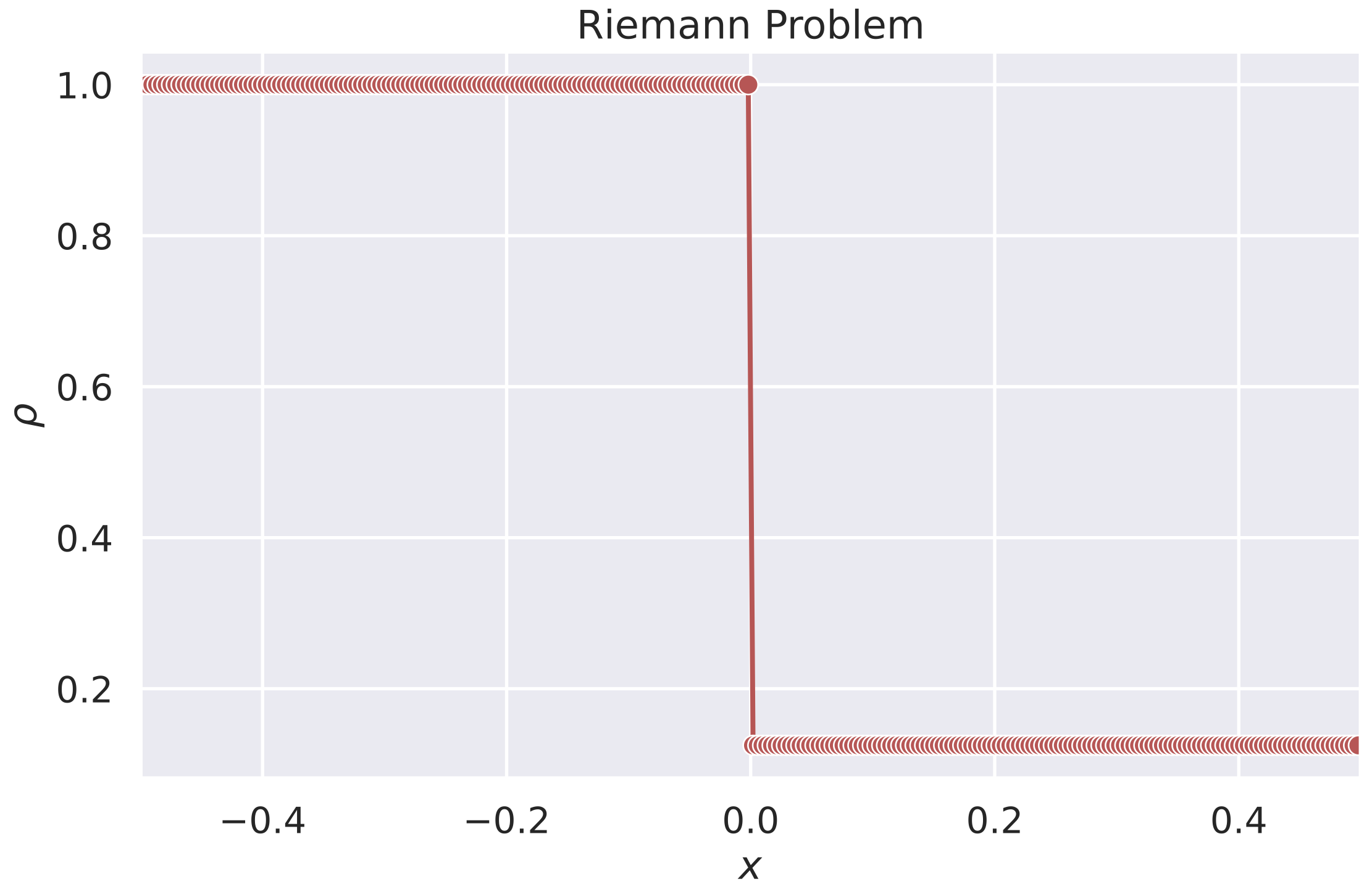
Hyperbolic conservation laws often turn smooth initial data into discontinuous solutions such as shocks and contact discontinuities. The Riemann problem is the simplest model of that behavior: a conservation law with a single jump in the initial data,

\[\mathbf{U}(x,0)= \begin{cases} \mathbf{U}_L, & x<0, \\ \mathbf{U}_R, & x>0. \end{cases}\]

Even though the initial condition is simple, its solution already contains the key mathematical structures that appear in shock-capturing methods and finite-volume solvers.

Mathematical setup

We consider a one-dimensional system of conservation laws

\[\frac{\partial \mathbf{U}}{\partial t} + \frac{\partial \mathbf{F}(\mathbf{U})}{\partial x} = 0,\]

where $\mathbf{U}$ is the vector of conserved variables and $\mathbf{F}(\mathbf{U})$ is the flux.

For the Riemann initial data above, the solution is often self-similar, meaning that it depends on $(x,t)$ only through

\[\xi = \frac{x}{t}, \qquad \mathbf{U}(x,t)=\widetilde{\mathbf{U}}(\xi), \qquad t>0.\]

Substituting this ansatz into the conservation law gives

\[-\xi \frac{d\widetilde{\mathbf{U}}}{d\xi} + \frac{d}{d\xi}\mathbf{F}(\widetilde{\mathbf{U}})=0.\]

If the solution is smooth at a given $\xi$, then with the Jacobian

\[A(\mathbf{U})=\frac{\partial \mathbf{F}}{\partial \mathbf{U}},\]

we obtain

\[\bigl(A(\widetilde{\mathbf{U}})-\xi I\bigr)\frac{d\widetilde{\mathbf{U}}}{d\xi}=0.\]

This is the basic equation behind the wave fan: nontrivial smooth variation can occur only when $\xi$ matches one of the characteristic speeds, i.e. one of the eigenvalues of $A(\mathbf{U})$.

Weak solutions and elementary waves

Because shocks are discontinuous, classical derivatives no longer make sense everywhere. The correct notion is a weak solution, which requires the conservation law to hold in integral form:

\[\int_0^\infty \int_{-\infty}^{\infty} \left( \mathbf{U}\,\phi_t + \mathbf{F}(\mathbf{U})\,\phi_x \right)\,dx\,dt + \int_{-\infty}^{\infty}\mathbf{U}(x,0)\phi(x,0)\,dx = 0\]

for every smooth test function $\phi$ with compact support.

The exact Riemann solution is built from three types of elementary waves.

1. Shock waves

Across a moving discontinuity with speed $s$, conservation implies the Rankine-Hugoniot condition

\[\mathbf{F}(\mathbf{U}_R)-\mathbf{F}(\mathbf{U}_L)=s(\mathbf{U}_R-\mathbf{U}_L).\]

This condition alone is not enough: nonphysical shocks can also satisfy it. To select the physically admissible branch, one imposes an entropy condition. For a compressive $k$-shock, a standard form is

\[\lambda_k(\mathbf{U}_L) > s > \lambda_k(\mathbf{U}_R).\]

In words, characteristics must enter the shock from both sides.

2. Rarefaction waves

A rarefaction is a continuous expanding wave. Inside a $k$-rarefaction,

\[\lambda_k(\mathbf{U})=\xi,\]

and the state varies along the corresponding eigenvector family:

\[\frac{d\mathbf{U}}{d\xi} \parallel \mathbf{r}_k(\mathbf{U}).\]

So rarefactions are governed by characteristic structure, not by jump conditions. They are the smooth parts of the wave fan.

3. Contact discontinuities

A contact discontinuity is associated with a linearly degenerate field,

\[\nabla \lambda_k(\mathbf{U}) \cdot \mathbf{r}_k(\mathbf{U}) = 0.\]

For the Euler equations, the contact moves with speed $u$. Across it, pressure and normal velocity remain continuous, while density may jump.

A concrete example: the 1D Euler equations

For an ideal gas, the one-dimensional Euler equations use the conserved variables

\[\mathbf{U}= \begin{pmatrix} \rho \\ \rho u \\ E \end{pmatrix}, \qquad \mathbf{F}(\mathbf{U})= \begin{pmatrix} \rho u \\ \rho u^2 + p \\ u(E+p) \end{pmatrix},\]

with equation of state

\[p=(\gamma-1)\left(E-\frac{1}{2}\rho u^2\right).\]

The sound speed is

\[c=\sqrt{\frac{\gamma p}{\rho}},\]

and the eigenvalues are

\[\lambda_1=u-c, \qquad \lambda_2=u, \qquad \lambda_3=u+c.\]

So the exact Euler Riemann solution contains three wave families: a 1-wave, a contact, and a 3-wave.

The Sod shock tube as the canonical example

The standard Sod shock tube uses

\[(\rho,u,p)_L=(1,0,1), \qquad (\rho,u,p)_R=(0.125,0,0.1), \qquad \gamma=1.4.\]

These states are physically admissible because both density and pressure are positive on each side.

For this problem, the exact solution has the familiar structure

a left rarefaction wave,
a contact discontinuity in the middle,
a right-moving shock wave.

The left and right initial states are not connected directly. Instead, one solves for intermediate star states separated by the contact. In practice, the exact Euler solver reduces to a nonlinear scalar equation for the intermediate pressure $p^\ast$, often solved by Newton iteration in the $p$-$u$ plane.

The important point is conceptual: the Riemann problem does not produce an arbitrary patchwork of states. Its structure is tightly constrained by characteristic speeds, Rankine-Hugoniot jumps, and entropy admissibility.

Why this matters numerically

Godunov-type finite-volume methods solve a local Riemann problem at every cell interface. If the reconstructed left and right states are

\[\mathbf{U}_{i+\frac{1}{2},\mathrm{L}}, \qquad \mathbf{U}_{i+\frac{1}{2},\mathrm{R}},\]

then the interface flux is obtained from the corresponding local wave interaction.

That is why the Riemann problem sits at the center of shock-capturing methods: it connects the analytical structure of hyperbolic PDEs to the numerical flux used in computation. A broader discussion of exact and approximate solvers is given in Riemann Solver.

A short note on MHD

The original version of this post tried to present the exact MHD Riemann problem in detail. That topic is significantly more delicate than the Euler case.

In one-dimensional ideal MHD, the exact fan can contain up to seven waves:

two fast magnetosonic waves,
two Alfvén waves,
two slow magnetosonic waves,
one contact discontinuity.

In a strictly one-dimensional setup, the normal magnetic field component $B_x$ is constant across the Riemann fan. Exact MHD solvers therefore require much more careful bookkeeping than Euler solvers, especially when handling degeneracies and intermediate states.

For a more accurate discussion of solver structure, see Riemann Solver and Numerical Methods for MHD - Part 3: Riemann Solvers.