Numerical Methods for MHD - Part 2: Numerical Methods and Solution Techniques

Posted Oct 4, 2024 Updated Mar 21, 2026

By Donghui Son 11 min read

Series Navigation

Numerical Methods for MHD
Solution Techniques for Scalar Equations

Notation note: Throughout this series, we keep $\mu_0$ explicit whenever magnetic terms appear. This part focuses on scalar model problems, but the notation stays consistent with the MHD parts.

3. Numerical Methods for MHD

Computational MHD often relies on discretizing partial differential equations in space and time. Two major approaches are finite difference (FD) and finite volume (FV) methods.

3.1 Finite Difference Methods

Finite difference methods (FD) approximate spatial and temporal derivatives using differences of field values at discrete grid points. They are conceptually simple and can achieve high order of accuracy on structured grids, but they may require special treatments (e.g., limiters) when dealing with strong shocks or discontinuities—common in MHD flows.

Basic derivative approximations (on a uniform 1D mesh with spacing $\Delta x$):

Forward Difference:
\[(\frac{\partial u}{\partial x})_{i} \approx \frac{u_{i+1} - u_i}{\Delta x}\]
Backward Difference:
\[(\frac{\partial u}{\partial x})_{i} \approx \frac{u_i - u_{i-1}}{\Delta x}\]
Central Difference:
\[(\frac{\partial u}{\partial x})_{i} \approx \frac{u_{i+1} - u_{i-1}}{2 \Delta x}\]

In practice, higher-order stencils or flux-limiter approaches may be used for improved accuracy and stability, particularly in shock-capturing schemes.

3.2 Finite Volume Methods

Finite volume methods (FV) are widely used for hyperbolic conservation laws like the MHD equations, as they directly enforce conservation in integral form and handle discontinuities naturally.

3.2.1 Core Idea

Divide the domain into small control volumes (cells), and apply the integral form of the conservation law to each cell:

\[\frac{\partial}{\partial t} \int_{V_i} U \, dV + \int_{\partial V_i} \mathbf{F}(U) \cdot \mathbf{n} \, dS = 0\]

$V_i$ : Volume of the $i$-th cell.
$\partial V_i$ : Boundary of the $i$-th cell.
$\mathbf{n}$ : Outward normal vector on each cell face

3.2.2 Discretization

Cell-Averaged Values:
\[\bar{U}_i = \frac{1}{V_i} \int_{V_i} U \, dV\]
Semi-Discrete Formulation:
\[\frac{d \bar{U}_i}{d t} = -\frac{1}{V_i} \sum_{faces} \left( \int_{face} \mathbf{F}(U) \cdot \mathbf{n} \, dS \right)\]
1D Example:
For uniform spacing $\Delta x$, the update formula simplifies to:
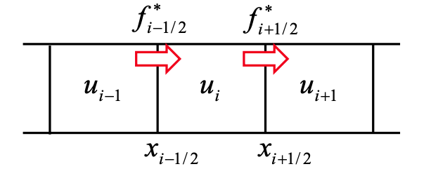
\[\frac{d \bar{U}_i}{d t} = -\frac{1}{\Delta x} \left( F_{i+\frac{1}{2}} - F_{i-\frac{1}{2}} \right)\]
where $F_{i+\frac{1}{2}}$ is the numerical flux at the interface between cells $i$ and $i+1$.

3.2.3 Computing Numerical Fluxes

At each interface, Godunov’s method sets up a Riemann problem between the left $\left(U_L\right)$ and right $\left(U_R\right)$ states.

Exact or Approximate Riemann Solvers can be used to solve for the flux:
\[F_{i+\frac{1}{2}} = \mathcal{R}(U_L, U_R)\]
Common approximate Riemann solvers: Roe, HLL, HLLC, HLLD (the latter specialized for MHD).

3.2.4 Advantages of Finite Volume Methods

Strict Conservation: Ensures mass, momentum, and energy are conserved at the discrete level.
Robust Shock Handling: Naturally captures strong discontinuities and shocks.
Flexibility: Works well on complex geometries and unstructured meshes.

3.2.5 Application to MHD Equations

Use conserved variables $U$ from the MHD system.
Compute fluxes $\mathbf{F}(U)$ at cell interfaces via Riemann solvers.
Preserve $\nabla \cdot \mathbf{B} = 0$ via divergence-control techniques (Constrained Transport, hyperbolic cleaning, etc.).

4. Solution Techniques for Scalar Equations

4.1 Linear Advection Equation

The linear advection equation models how a scalar quantity $u(x, t)$ moves with a constant speed $a$:

\[\frac{\partial u}{\partial t} + a \frac{\partial u}{\partial x} = 0, \quad a > 0 \ (const)\]

This PDE governs the transport of waves or signals without changing their shape, which is useful in modeling phenomena such as sound waves or simple transport processes.

Analytical Solution

For an initial condition $u_{0}(x)$ at $t = 0$, the solution is:

\[u(x, t) = u_{0}(x - a t)\]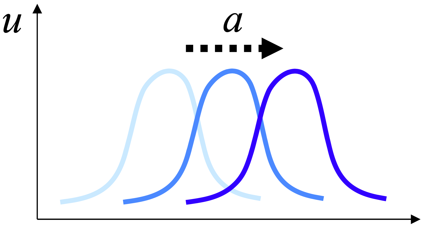

Numerical Methods

Key challenge: Capturing the wave’s motion accurately while maintaining stability and minimizing numerical diffusion or oscillations.

Upwind Scheme: Leverages the direction of propagation to ensure information flows from upstream cells
\[u_i^{n+1} = u_i^n - \frac{a \Delta t}{\Delta x} (u_i^n - u_{i-1}^n)\]
1 2 3 4 5 def upwind_scheme_periodic(u, a, dt, dx): c = a * dt / dx if a >= 0: return u - c * (u - np.roll(u, 1)) return u - c * (np.roll(u, -1) - u)
- Pros: Simple, stable in one dimension if the CFL condition is satisfied.
- Cons: Only first-order accurate; can be more diffusive in smooth regions.
Stability Condition: CFL Numerical stability requires the Courant-Friedrichs-Lewy (CFL) condition:
\[\frac{a \Delta t}{\Delta x} \leq 1\]
1 2 def check_cfl(a, dt, dx): return a * dt / dx <= 1
This ensures the wave cannot “jump” over more than one grid cell per time step.
Lax-Friedrichs Scheme: A more diffusive scheme, which helps stabilize solutions by averaging neighboring states:
\[u_i^{n+1} = \frac{1}{2} (u_{i+1}^n + u_{i-1}^n) - \frac{a \Delta t}{2 \Delta x} (u_{i+1}^n - u_{i-1}^n)\]
1 2 def lax_friedrichs_scheme(u, a, dt, dx): return 0.5 * (u[2:] + u[:-2]) - 0.5 * (a * dt / dx) * (u[2:] - u[:-2])
- Interpretation: Half of the new state is an average of neighbors (smoothing), while the other half accounts for advection.
- Pros: Very robust, less prone to oscillations near discontinuities.
- Cons: Excess numerical diffusion can smear out sharp features.

4.2 Nonlinear Advection Equation (Inviscid Burgers’ Equation)

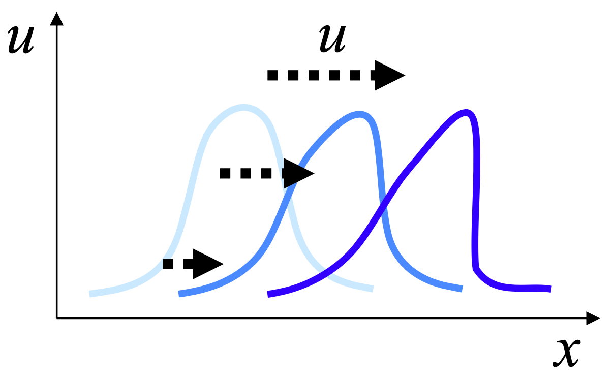
The inviscid Burgers’ equation adds a nonlinear advection term:

\[\frac{\partial u}{\partial t} + u \frac{\partial u}{\partial x} = 0.\]

Commonly used to model shock waves, traffic flow, and other nonlinear wave phenomena.
Nonlinearity means wave characteristics can merge, producing shocks.

Upwind Scheme for Nonlinear Equation

Burgers’ equation can be written in conservation form with flux $f(u) = \frac{1}{2} u^2$. A straightforward finite volume update is:

\[u_i^{n+1} = u_i^n - \frac{\Delta t}{\Delta x} (f_{i+\frac{1}{2}} - f_{i-\frac{1}{2}}).\]

Determine Upwind Direction: For Burgers’ equation, the relevant speed is the interface characteristic speed $f’(u)=u$, so the left state is upwind when the characteristic speed is positive and the right state is upwind when it is negative.
\[\begin{cases} f(u_L) & \text{is used at an interface if the local wave speed is positive}, \\ f(u_R) & \text{is used at an interface if the local wave speed is negative}. \end{cases}\]
In transonic cases, such as $u_L \le 0 \le u_R$, one should use an entropy-satisfying numerical flux (e.g., the Godunov flux) rather than choosing the direction from a single cell-centered value.
Shock Formation:
- When characteristics converge, waveforms steepen and form discontinuities (shocks).
- An entropy condition is needed to ensure the physically correct shock solution (rather than a rarefaction).

4.3 Method of Characteristics

Characteristics give a powerful analytic framework to understand wave propagation:

Linear Advection $(a > 0)$
\[\frac{\partial u}{\partial t} + a \frac{\partial u}{\partial x} = 0.\]
- Characteristic Equations
  \[\frac{dx}{dt} = a, \quad \frac{du}{dt} = 0.\]
  Along lines $x = x_0 + a t$, $u$ remains constant.
Burgers’ Equation
\[\frac{\partial u}{\partial t} + u \frac{\partial u}{\partial x} = 0.\]
- Characteristic Equations
  \[\frac{dx}{dt} = u, \quad \frac{du}{dt} = 0\]
  Since $u$ is constant along characteristics, the wave speed itself depends on $u$. Intersections of characteristics lead to shock formation.

In linear problems, characteristic paths never intersect; the wave profile simply translates. By contrast, in nonlinear problems such as Burgers’, characteristic convergence causes discontinuities that demand careful numerical treatment and shock capturing methods.

Example 1: Solving the Linear Advection Equation

We consider the PDE:

\[\frac{\partial u}{\partial t} + a \frac{\partial u}{\partial x} = 0, \quad a > 0 \ (const),\]

on the periodic domain $x \in [0, L)$, where the endpoint is excluded so that the grid does not duplicate both $x=0$ and $x=L$. Here’s a Python implementation of the upwind scheme, along with a simple function to animate the solution.

  
import numpy as np
import matplotlib.pyplot as plt
import seaborn as sns
from matplotlib.animation import FuncAnimation, PillowWriter
from IPython.display import HTML

# 1) Use Seaborn for nice plot aesthetics
sns.set_theme(style="darkgrid")

def upwind_scheme(u, a, dt, dx):
    """
    Applies a 1D periodic upwind scheme to all grid points.
    """
    c = a * dt / dx
    if a >= 0:
        return u - c * (u - np.roll(u, 1))
    return u - c * (np.roll(u, -1) - u)

def solve_linear_advection(u0, a, T, L, Nx, Nt):
    """
    Solves the linear advection equation over the periodic domain [0,L).
    - u0: function returning the initial condition
    - a: advection speed
    - Nx: number of spatial cells
    - Nt: number of time steps
    Returns x, t, and the solution array u of shape (Nt + 1, Nx).
    """
    dx, dt = L / Nx, T / Nt
    x = np.linspace(0, L, Nx, endpoint=False)
    t = np.linspace(0, T, Nt + 1)

    # 2D array to store solution at each time step
    u = np.zeros((Nt + 1, Nx))
    u[0] = u0(x)  # Initialize solution at t=0

    for n in range(Nt):
        u[n + 1] = upwind_scheme(u[n], a, dt, dx)

    return x, t, u

def create_animation(x, t, u, L):
    """
    Creates a Matplotlib animation of the solution over time.
    """
    fig, ax = plt.subplots(figsize=(12, 7))
    line, = ax.plot([], [], lw=2.5, color=sns.color_palette("husl", 8)[0])

    ax.set_xlim(0, L)
    ax.set_ylim(0, 1.1)
    ax.set_xlabel('x', fontsize=14)
    ax.set_ylabel('u', fontsize=14)
    ax.set_title('Linear Advection Equation Solution', fontsize=16)
    ax.tick_params(axis='both', labelsize=12)

    # Optional: add a light gradient background
    gradient = np.linspace(0, 1, 256).reshape(1, -1)
    ax.imshow(gradient, extent=[0, L, 0, 1.1], aspect='auto', alpha=0.1, cmap='coolwarm')

    def init():
        line.set_data([], [])
        return line,

    def animate(i):
        line.set_data(x, u[i])
        ax.set_title(f'Linear Advection (t = {t[i]:.2f})', fontsize=16)
        return line,

    return FuncAnimation(fig, animate, init_func=init, frames=len(t), interval=50, blit=True)

# Parameters and initial condition
L, T = 1.0, 1.0       # Domain length and final time
Nx, Nt = 200, 200     # Grid and timestep counts
a = 1.0               # Constant advection speed

# Gaussian-like initial condition centered at x=L/4
u0 = lambda x: np.exp(-((x - L/4)**2) / 0.01)

# 1) Solve the equation
x, t, u = solve_linear_advection(u0, a, T, L, Nx, Nt)

# 2) Animate the solution
anim = create_animation(x, t, u, L)

# 3) Save the animation as a GIF
writer = PillowWriter(fps=15)
anim.save('linear_advection_animation_seaborn.gif', writer=writer, dpi=100)

# 4) Display the animation in a Jupyter notebook
plt.close(anim._fig)  # Close the figure before displaying
HTML(anim.to_jshtml())

Key Points

Upwind Scheme:
This first-order method is stable as long as the CFL condition, $\frac{a \Delta t}{\Delta x} \leq 1$, is satisfied.
Periodic Boundaries:
We use endpoint=False and np.roll(...) so that the periodic wrap-around is handled consistently at every grid point.
Visualization:
The code leverages matplotlib.animation to show the solution evolving over time, verifying that the initial Gaussian profile simply translates to the right.

Example 2: Solving the Viscous Burgers’ Equation

\[\frac{\partial u}{\partial t} + u \frac{\partial u}{\partial x} = \nu \frac{\partial^2 u}{\partial x^2},\]

where $\nu$ is the viscosity coefficient. This PDE balances nonlinear advection against diffusion, resulting in smoother wavefronts compared to the inviscid case.

Physical Interpretation:
- Nonlinear Advection $\left(u \frac{\partial u}{\partial x}\right)$ can steepen wavefronts.
- Diffusion $\left(\nu \frac{\partial^2 u}{\partial x^2}\right)$ smoothes out gradients, preventing shock singularities.
- By varying $\nu$, one transitions from nearly inviscid, shock-like solutions to more diffuse, parabolic-like profiles.
Numerical Scheme
A simple explicit finite-difference approach:
- Advection term: upwind or flux-based difference
- Diffusion term: second-order central difference

A common discretized update for each interior cell $i$ can look like:

\[u_i^{n+1} = u_i^n - \Delta t \left(\text{advection}_{i}^{n}\right) + \Delta t \left(\text{diffusion}_{i}^{n}\right),\]

where:

\[\begin{cases} \text{advection}_{i}^{n} & \approx \frac{1}{\Delta x} \left( F(u_{i}^{n}) - F(u_{i-1}^{n}) \right) \text{with } F(u) = u^2/2, \\ \text{diffusion}_{i}^{n} & \approx \nu \frac{\left( u_{i+1}^{n} - 2u_{i}^{n} + u_{i-1}^{n} \right)}{\Delta x^2}. \end{cases}\]

Stability Condition typically requires:

A CFL-like condition for the advection part: $\frac{u_{max}\Delta t}{\Delta x} \leq 1$,
A diffusive condition: $\nu \frac{\Delta t}{\Delta x^2} \leq \frac{1}{2}$ (for explicit methods).

References

R. J. LeVeque, Finite Volume Methods for Hyperbolic Problems, Cambridge University Press, 2002.
E. F. Toro, Riemann Solvers and Numerical Methods for Fluid Dynamics, 3rd ed., Springer, 2009.
C.-W. Shu and S. Osher, “Efficient implementation of essentially non-oscillatory shock-capturing schemes,” Journal of Computational Physics 77 (1988), 439-471.

Computational MHD, Introduction

This post is licensed under CC BY 4.0 by the author.