Numerical Methods for MHD - Part 4: Advanced Topics

Posted Oct 6, 2024 Updated Mar 21, 2026

By Donghui Son 18 min read

Series Navigation

Advanced Topics and Practical Implementation

Notation note: Throughout this series, we keep $\mu_0$ explicit. If you work in normalized MHD units, the same formulas can be converted to the $\mu_0 = 1$ convention after nondimensionalization.

6. Advanced Topics and Practical Implementation

6.1 Advanced Numerical Techniques

6.1.1. High-Order Spatial Reconstruction

Accurate and stable solutions of conservation laws (e.g., the Euler or MHD equations) often require schemes of at least second or third order in space. Godunov-type methods rely on cell-interface fluxes computed from reconstructed values of the solution. Below we describe two powerful reconstruction strategies: WENO and MP.

WENO Reconstruction (Weighted Essentially Non-Oscillatory)
- Motivation and Overview
  - Key Goal: Achieve high-order accuracy in smooth regions of the flow while avoiding Gibbs-like oscillations near shocks or discontinuities.
  - Foundational Idea: WENO uses a weighted combination of several candidate stencils. The method assigns small weights to stencils containing discontinuities (where the solution is less smooth) and larger weights to smooth stencils, effectively “turning off” problematic stencils that might cause oscillations.
- 1D Example: WENO-JS (fifth-order)
  Consider a fifth-order WENO scheme reconstructing the value $u_{i+\frac{1}{2}}$ at the right interface of cell $i$. We form a polynomial approximation from three sub-stencils $\left(S_0, S_1, S_2\right)$, each of width $3$ points. Typically, the sub-stencils might be:
  - $S_0$ uses grid cells $\left( i-2, i-1, i \right)$
  - $S_1$ uses grid cells $\left( i-1, i, i+1 \right)$
  - $S_2$ uses grid cells $\left( i, i+1, i+2 \right)$
  Each sub-stencil builds a third-order polynomial, denoted $P_0$, $P_1$, $P_2$. Then WENO combines these polynomials into a single approximation of the interface value $u_{i+\frac{1}{2}}$.
  - Candidate Polynomials:
    \[P_k(x), \quad k = 0, 1, 2\]
    each approximates the solution based on cells in sub-stencil $S_k$.
  - Smoothness Indicators:
    To detect which sub-stencil is “smooth” and which contains steep gradients, WENO computes smoothness indicators $\beta_k$. One classical choice (Jiang & Shu) is:
    \[\beta_k = \sum_{m=1}^{2} \int_{x_{i-1/2}}^{x_{i+1/2}} \Delta x^{\,2m-1} \left( \frac{d^m}{dx^m} P_k(x) \right)^2 dx,\]
    where each term measures how large the polynomial derivatives are over the cell. In practice, these integrals reduce to discrete finite-difference formulas.
    Example: A standard set in the WENO-JS literature.
    \[\begin{aligned} \beta_0 &= \frac{13}{12} \bigl(u_{i-2}-2\,u_{i-1}+u_i\bigr)^2 + \frac{1}{4} \bigl(u_{i-2}-4\,u_{i-1}+3\,u_i\bigr)^2, \\ \beta_1 &= \frac{13}{12} \bigl(u_{i-1}-2\,u_i + u_{i+1}\bigr)^2 + \frac{1}{4} \bigl(u_{i-1}-u_{i+1}\bigr)^2, \\ \beta_2 &= \frac{13}{12} \bigl(u_i -2\,u_{i+1} + u_{i+2}\bigr)^2 + \frac{1}{4} \bigl(3\,u_i -4\,u_{i+1} + u_{i+2}\bigr)^2. \end{aligned}\]
  - Linear (Ideal) Weights
    If the flow is smooth over the entire $5$-point stencil, a straightforward third-order upwind scheme would combine these sub-stencils with fixed weights $d_k$. For example, a known set of linear weights for WENO-JS is:
    \[\left( d_0, d_1, d_2 \right) = \left( \tfrac{1}{10}, \tfrac{6}{10}, \tfrac{3}{10} \right).\]
    Then one might linearly combine:
    \[P_{\mathrm{linear}}(x_{i+\tfrac12}) = \sum_{k=0}^{2} d_k\,P_k\bigl(x_{i+\tfrac12}\bigr).\]
    However, near discontinuities, the polynomial containing the discontinuity would cause Gibbs-like oscillations. WENO solves this via nonlinear weights that downweight sub-stencils crossing discontinuities.
  - Nonlinear Weights $\left(\omega_k\right)$
    Let $d_k$ be the ideal weight for sub-stencil $k$ (the fraction used in purely smooth flow). Then define:
    \[\alpha_k = d_k \;\bigl(\epsilon + \beta_k\bigr)^{-p},\]
    where $\epsilon\sim 10^{-6} \text{ to } 10^{-40}$ avoids division by zero, and $p\ge 1$ is often set to 2. The factor $(\beta_k)^{-p}$ downweights stencils with large $\beta_k$ (i.e., a discontinuity or large gradient).
    Normalized weights are then:
    \[\omega_k = \frac{\alpha_k}{\sum_{j=0}^2 \alpha_j}.\]
    This ensures $\sum_{k=0}^2 \omega_k = 1$. If one stencil is near a discontinuity, its $\beta_k$ is large, making $\alpha_k$ small, thus $\omega_k\approx 0$.
  - Final WENO-JS Reconstruction:
    The reconstructed interface value at $x_{i+\tfrac12}$ is:
    \[u_{i+\tfrac12}^{\mathrm{WENO}} = \sum_{k=0}^{2} \omega_k P_k\bigl(x_{i+\tfrac12}\bigr).\]
    Because at least one sub-stencil remains smooth, the final polynomial retains high-order accuracy in smooth regions. Near discontinuities, the solver automatically biases toward the sub-stencils that remain smooth, preventing large oscillations.
[!NOTE]
Above we described a left-biased reconstruction for the right cell interface. For compressible flow or MHD, we similarly define a right-biased WENO for the left interface (i.e., reconstructing $u_{i-1/2}$).
MP Reconstruction (Monotonicity Preserving):
Monotonicity-preserving (MP) schemes aim to achieve high-order accuracy in smooth regions while respecting the monotonicity of the solution near discontinuities or steep gradients. Unlike total-variation-diminishing (TVD) schemes that often restrict the scheme to second-order accuracy, MP schemes can maintain higher-order accuracy (e.g., fifth order) without introducing unphysical oscillations.
- Motivation and Overview
  - TVD/Second-Order Limitation: Classical TVD (Total Variation Diminishing) methods are robust but typically limited to second-order accuracy in smooth regions.
  - Monotonicity-Preserving Idea: MP extends these concepts by adapting higher-order polynomials (third-, fourth-, or fifth-order) but applies slope limiters or correction terms in a way that prevents any new local extrema from appearing in the reconstructed solution.
- Basic Principle
  - Generate a base high-order polynomial reconstruction (e.g., 5th-order).
  - Apply a monotonicity-preserving limiter that adjusts the polynomial only if it would create new extrema (i.e., overshoot or undershoot neighboring cell values).
  Thus, in smooth parts of the solution, the scheme retains full higher-order accuracy; near discontinuities, it smoothly transitions to a more limited shape, avoiding spurious oscillations.
- 1D Example: MP5 (fifth-order)
  We illustrate a fifth-order monotonicity-preserving scheme, commonly called MP5.
  - Polynomial Construction
    - Stencil: A common approach uses a 5-point stencil $(u_{i-2}, u_{i-1}, u_i, u_{i+1}, u_{i+2})$ around a cell index $i$.
    - Fifth-Order Polynomial: Denote a polynomial $P_i(x)$ of degree 4 that interpolates or approximates these five points. In a finite-volume setting, one might reconstruct interface values $u_{i\pm\tfrac12}$; in a finite-difference setting, we might approximate pointwise solutions.
    For uniform mesh spacing $\Delta x$, let $x_i = x_0 + i\,\Delta x$. We often define a local coordinate $\xi = (x - x_i)/\Delta x$, so $\xi \in [-0.5, +0.5]$ if reconstructing to the left or right interface.
    - Preliminary High-Order Approximation
      We compute a standard fifth-order polynomial using standard finite-difference formulas (e.g., a 5th-order central scheme). Denote this preliminary interface value as $u_{i+\tfrac12}^{(5)}$.
  - MP limiter
    MP5 modifies $u_{i+\tfrac12}$ if it introduces new local extrema. Specifically:
    - Compute Slopes
      Let
      \[d_i = \frac{u_{i+1} - u_{i-1}}{2}, \quad d_{i+1} = \frac{u_{i+2} - u_i}{2},\]
      or other representative slopes. We also define limited slopes like
      \[d_{i,\mathrm{minmod}} = \mathrm{minmod}(u_i - u_{i-1},\,u_{i+1} - u_i),\]
      to ensure we capture the local monotonicity.
    - Detecting Non-Monotonic Behavior
      The scheme checks if the polynomial reconstruction at $x_{i+\tfrac12}$ or $x_{i-\tfrac12}$ overshoots the local maxima or undershoots the local minima in neighboring cells. For instance, if
      \[u_{i+\tfrac12}^{(5)} > \max\bigl(u_i,u_{i+1}\bigr) + \epsilon \quad\text{or}\quad u_{i+\tfrac12}^{(5)} < \min\bigl(u_i,u_{i+1}\bigr) - \epsilon,\]
      then the scheme triggers a slope adjustment.
    - Monotonicity-Preserving Correction
      A typical form is
      \[u_{i+\tfrac12} = u_{i+\tfrac12}^{(5)} - \Theta_i \,\bigl[u_{i+\tfrac12}^{(5)} - u_{i+\tfrac12}^{(\mathrm{lower-order})}\bigr],\]
      where $u_{i+\tfrac12}^{(\mathrm{lower-order})}$ is a more robust, lower-order approximation (often second- or third-order).
      $\Theta_i\in[0,1]$ is chosen to clamp the solution if it violates monotonicity:
      \[\Theta_i = \phi\bigl(\Delta_{i}, \Delta_{i+1}, \dots\bigr),\]
      for some limiting function $\phi$. The result is that the final interface value remains within the cell-average bounds of $u_i, u_{i+1}$.
    Minmod or van Leer-type limiters are often integrated into MP logic to ensure the final slope is consistent with neighboring cells.
    - Concrete Formulas (Suresh & Huynh)
      In the classic MP5 formulation:
      - Base Fifth-Order Approximation
        \[u_{i+\tfrac12}^{(5)} = \tfrac{1}{60} \Bigl( 2\,u_{i-2} - 13\,u_{i-1} + 47\,u_{i} + 27\,u_{i+1} - 3\,u_{i+2} \Bigr).\]
        (One-sided variations exist near boundaries.)
      - Second-Order Backup
        \[u_{i+\tfrac12}^{(\mathrm{2nd})} = \tfrac12 \bigl(u_i + u_{i+1}\bigr) - \tfrac{1}{8} \bigl(u_{i+1} - u_i\bigr).\]
        (This is a standard limited linear slope.)
      - Monotonicity-Preserving Check
        If $u_{i+\tfrac12}^{(5)}$ is “safe” (no new extrema formed), keep it. Otherwise, blend it toward $u_{i+\tfrac12}^{(\mathrm{2nd})}$ More advanced codes define a function $\mathrm{MP_limit}(u_{i+\tfrac12}^{(5)}, u_{i+\tfrac12}^{(\mathrm{2nd})}, u_i, u_{i+1}, \dots)$ that systematically adjusts the interface value.
        Various detailed formulas in the Suresh & Huynh paper or in open-source CFD codes (e.g., Athena, PLUTO) show exactly how to enforce constraints like:
        \[\min(u_i,u_{i+1}) \;\le\; u_{i+\tfrac12} \;\le\; \max(u_i,u_{i+1}),\]
        and no overshoots with respect to $u_{i-1}, u_{i+2}$, etc.
- Accuracy and Properties
  - High Order: In smooth regions, MP5 maintains fifth-order accuracy, as the limiting function $\Theta_i$ remains close to 0 if no discontinuity is detected.
  - Monotonicity: Near steep gradients, it lowers the effective order (often ~2nd or 3rd) locally to prevent oscillations.
  - Total Variation: MP schemes typically do not strictly guarantee TVD in the traditional sense (like second-order TVD methods), but in practice, they produce bounded or very low numerical oscillations.
- Implementation Outline
  A typical MP reconstruction step for each interface $x_{i+\tfrac12}$ might be:
  - Compute the base polynomial $u_{i+\tfrac12}^{(5)}$ using a central 5-point formula or upwind 5-point formula.
  - Compute a fallback $u_{i+\tfrac12}^{(\mathrm{low})}$ (often 2nd-order or 3rd-order).
  - Check monotonicity:
    - If $u_{i+\tfrac12}^{(5)}$ violates monotonicity w.r.t. neighboring cell values, apply the MP limiter:
      \[u_{i+\tfrac12} = u_{i+\tfrac12}^{(5)} - \Theta_i \,\bigl[u_{i+\tfrac12}^{(5)} - u_{i+\tfrac12}^{(\mathrm{low})}\bigr].\]
    - Otherwise, do nothing (retain the original 5th-order value).
  - Use $u_{i+\tfrac12}$ as left or right state for the Riemann solver (depending on direction of reconstruction).
  Boundary and corner cells might need specialized stencils or one-sided formulas to maintain overall stability.
- Relationship to Other Methods
  - TVD: Monotonicity-preserving can be viewed as a natural extension of TVD to higher orders.
  - WENO: Both WENO and MP aim to avoid oscillations.
    - WENO adaptively selects stencils,
    - MP keeps a single polynomial but uses slope limiting.

6.1.2 Time Integration Methods

Robust time integration is essential for ensuring accuracy and stability in numerical simulations of hyperbolic PDEs (e.g., Euler equations, MHD). This section highlights Strong Stability Preserving (SSP) Runge–Kutta methods, which help maintain desirable stability properties—particularly Total Variation Diminishing (TVD)—under certain time step constraints.

A) Strong Stability Preserving (SSP) Runge–Kutta Methods

Motivation
When solving PDEs with discontinuities (like shocks), one often wants a numerical scheme that does not increase the total variation of the solution. This avoids spurious oscillations and preserves monotonicity near shocks or steep gradients. SSP Runge–Kutta methods (formerly called TVD Runge–Kutta) extend the concept of TVD from simple forward Euler steps to multi-stage time discretizations.
Key Idea
- Each stage of the Runge–Kutta update is formed by a convex combination of “forward Euler” steps that individually satisfy the stability property (e.g., TVD).
- The final result is a higher-order method in time that preserves the underlying non-oscillatory character of the spatial discretization, as long as the time step $\Delta t$ meets a certain CFL-type constraint.
Total Variation Diminishing (TVD) Property
- A scheme is TVD if the total variation of the numerical solution does not grow:
\[TV(u^{n+1}) \;\le\; TV(u^n).\]
- SSP Runge–Kutta methods ensure this property (or a closely related non-oscillatory criterion) is preserved at each stage, provided the time step is sufficiently small.
General Formulation
An $s$-stage SSP Runge–Kutta method updates a solution $u^n$ to $u^{n+1}$ as follows:
\[\begin{aligned} u^{(1)} &= u^n \;+\; \Delta t \,L\bigl(u^n\bigr),\\ u^{(2)} &= \alpha_2 \,u^n \;+\; \beta_2 \,u^{(1)} \;+\;\Delta t \,L\bigl(u^{(1)}\bigr),\\ &\quad \vdots \\ u^{(s)} &= \alpha_s \,u^n \;+\; \beta_s \,u^{(s-1)} \;+\;\Delta t \,L\bigl(u^{(s-1)}\bigr),\\ u^{n+1} &= u^{(s)}, \end{aligned}\]
where:
- $L(u)$ represents the spatial discretization (e.g., flux difference for finite volumes).
- Coefficients $\left(\alpha_i,\beta_i\right)$ are chosen to ensure the SSP property—each stage remains a convex combination of TVD-like updates.
Time Step Constraints
- Just like simple forward Euler methods, SSP schemes come with a maximum allowed $\Delta t$ that depends on the Courant–Friedrichs–Lewy (CFL) condition.
- If $\Delta t$ is too large, the scheme may lose its TVD or non-oscillatory guarantee. Ensuring $\Delta t$ is within bounds maintains the strong stability.

B) Example: SSPRK(3,3)

A popular three-stage, third-order SSP Runge–Kutta scheme is given by:

\[\begin{aligned} u^{(1)} &= u^n + \Delta t \cdot L\bigl(u^n\bigr),\\ u^{(2)} &= \tfrac34\,u^n + \tfrac14\,\Bigl(u^{(1)} + \Delta t \cdot L\bigl(u^{(1)}\bigr)\Bigr),\\ u^{(3)} &= \tfrac13\,u^n + \tfrac23\,\Bigl(u^{(2)} + \Delta t \cdot L\bigl(u^{(2)}\bigr)\Bigr),\\ u^{n+1} &= u^{(3)}. \end{aligned}\]

Stage-by-Stage Breakdown

Stage 1:
$u^{(1)} = u^n \;+\;\Delta t \,L\bigl(u^n\bigr).$
Stage 2:
$u^{(2)} = \tfrac34\,u^n + \tfrac14\bigl(u^{(1)} + \Delta t\,L(u^{(1)})\bigr).$
Stage 3:
$u^{(3)} = \tfrac13\,u^n + \tfrac23\bigl(u^{(2)} + \Delta t\,L(u^{(2)})\bigr).$
Final Update:
$u^{n+1} = u^{(3)}.$

This SSPRK(3,3) method is third-order accurate in time and preserves the strong stability (TVD-like) property under a suitably chosen time step. It’s widely used in shock-capturing schemes paired with non-oscillatory spatial discretizations (e.g., WENO, MP).

A genuine four-stage, third-order SSPRK scheme uses a different set of coefficients; such variants are often chosen to enlarge the allowable CFL number, but they are not the same method written above.

C) Summary and Practical Notes

Preserving Non-Oscillatory Behavior: SSP methods ensure that if the spatial discretization is non-oscillatory (TVD) under forward Euler, then the multi-stage integration remains non-oscillatory.
Order and Stages: Higher-order SSP RK schemes typically require more stages, and there’s a known trade-off between the achievable order, the number of stages, and the size of the stable time step.
Implementation: Straightforward to implement by chaining partial updates, as in standard RK. Just ensure the coefficients $\left(\alpha_i, \beta_i\right)$ reflect the particular SSP scheme you want.
Applications: Common in finite-volume or finite-difference codes for compressible flows, MHD, shallow water, etc., where controlling oscillations around discontinuities is critical.

Thus, SSP Runge–Kutta methods form a robust backbone for time integration in high-resolution shock-capturing methods, ensuring that carefully designed spatial discretizations (e.g., WENO, MP) retain their non-oscillatory properties.

6.1.3 Maintaining Divergence-Free Magnetic Fields

In ideal MHD, the condition $\nabla \cdot \mathbf{B} = 0$ must hold at all times. Numerically, failing to preserve this leads to non-physical artifacts (e.g., artificial forces, negative pressures). Below are two widely used strategies—Constrained Transport (CT) and Hyperbolic Divergence Cleaning—to maintain or restore the $\nabla\cdot\mathbf{B}=0$ condition in a discrete setting.

A) Constrained Transport (CT)

1. Motivation and Core Idea

Faraday’s Law in ideal MHD (omitting resistive terms) is
\[\frac{\partial \mathbf{B}}{\partial t} + \nabla \times (\mathbf{E}) = 0,\]
or equivalently
\[\frac{\partial \mathbf{B}}{\partial t} = -\nabla \times (\mathbf{E}).\]
CT discretizes this in such a way that magnetic flux is conserved exactly from one time step to the next, keeping $\nabla \cdot \mathbf{B} = 0$ at machine precision.

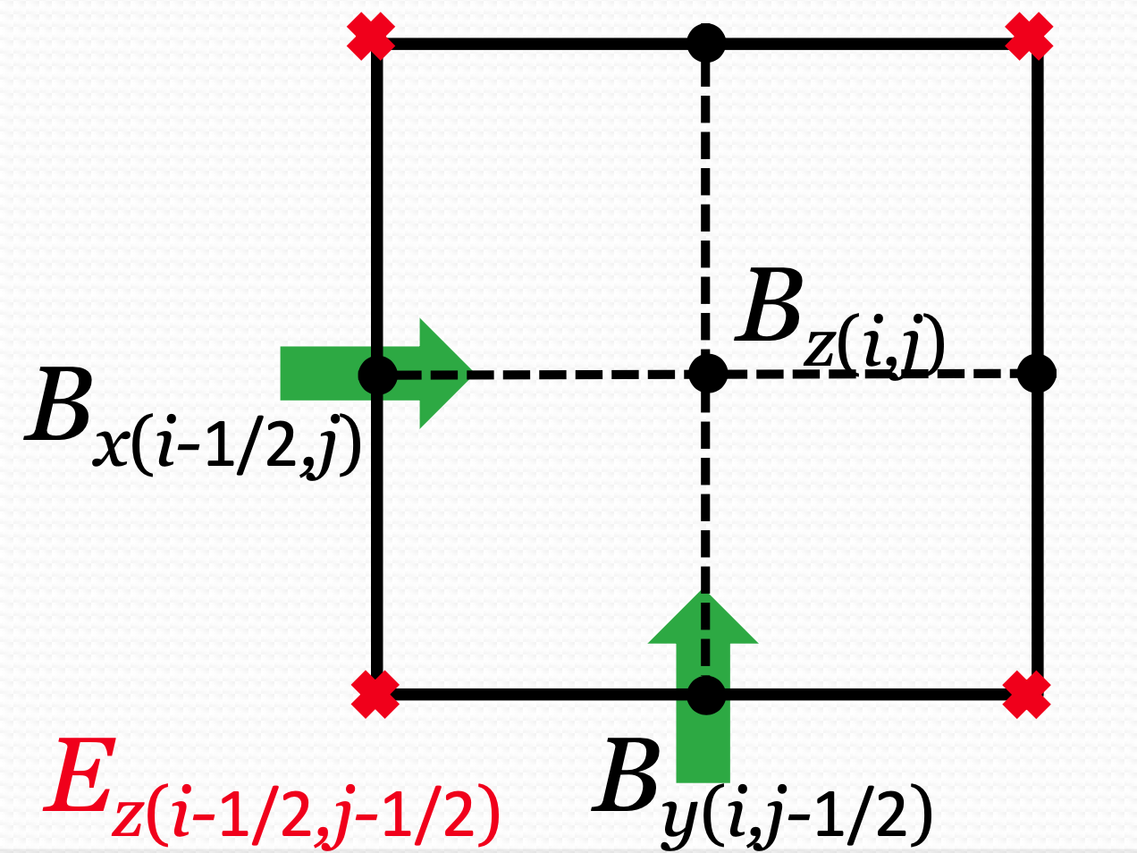
2. Staggered Grid Layout

Magnetic field components $\left(B_x, B_y, B_z\right)$ are stored on cell faces.
Electric field components $\left(E_x, E_y, E_z\right)$ are stored on cell edges.
Cell-centered values typically represent other quantities like density or velocity.

This positioning allows discrete curl and divergence operations to be computed in a flux-consistent manner.

3. Discrete Induction Equation

Starting from

\[\frac{\partial \mathbf{B}}{\partial t} = - \nabla \times (\mathbf{E}),\]

we integrate over a cell face to track magnetic flux. For example, for the $B_x$ component on a face normal to the x-direction:

Continuous Form:
\[\frac{\partial}{\partial t} \int_{\text{face}} B_x \, dA = - \int_{\text{face}} (\nabla \times E)_x \, dA.\]
Converting the right side to a line integral around the cell face via Stokes’ theorem yields integrals of $E_z$ and $E_y$.
Discrete Update:
\[\begin{aligned} B_x^{n+1}(i,j,k) = B_x^n(i,j,k) &- \left(\Delta t / \Delta y\right)\left[ E_z^{n+1/2}(i, j+1/2, k) - E_z^{n+1/2}(i, j-1/2, k) \right] \\ &+ \left(\Delta t / \Delta z\right)\left[ E_y^{n+1/2}(i, j, k+1/2) - E_y^{n+1/2}(i, j, k-1/2) \right]. \end{aligned}\]
This ensures exact flux balance for $\mathbf{B}$ through the appropriate cell faces. Similar expressions apply for $B_y$ and $B_z$.

4. Preserving $\nabla \cdot \mathbf{B}$

Because each face’s flux update is computed from circulations of $\mathbf{E}$ at edges, the net magnetic flux around a closed surface cancels out exactly. This guarantees
\[\nabla \cdot \mathbf{B}^{n+1} = 0.\]
in the discrete sense.

5. Practical Implementation

One must consistently interpolate or reconstruct $E_x, E_y, E_z$ at edges using the velocity $\mathbf{v}$ and $\mathbf{B}$ from adjacent cells ($\mathbf{E} = - \mathbf{v} \times \mathbf{B}$ in ideal MHD).
CT is used in many MHD codes (e.g., Athena, PLUTO, FLASH) to maintain a rigorous control of magnetic field divergence.

B) Hyperbolic Divergence Cleaning

1. Extended MHD Equations

A common formulation (Dedner et al., 2002) augments the induction equation with a scalar potential $\psi$:

\[\frac{\partial \mathbf{B}}{\partial t} + \nabla \cdot (\mathbf{v} \otimes \mathbf{B} - \mathbf{B} \otimes \mathbf{v} + \psi \mathbf{I}) = 0,\] \[\frac{\partial \psi}{\partial t} + c_h^2 \nabla \cdot \mathbf{B} = - \left(\frac{c_h^2}{c_p^2}\right) \psi.\]

$ c_h $: Hyperbolic cleaning speed (controls how fast divergence errors propagate out).
$ c_p $: Parabolic damping or damping speed (exponential decay rate of $\psi$).

2. Mechanism

Propagation: Any non-zero $\nabla \cdot \mathbf{B}$ induces a non-zero $\psi$, which in turn modifies $\mathbf{B}$ so that errors are carried away at speed $c_h$.
Damping: The second equation forces $\psi \to 0$ on a timescale $(c_p^2 / c_h^2)$, damping the divergence-related potential.
Over time, this “cleaning wave” flushes out spurious divergence, leaving $\mathbf{B}$ nearly solenoidal.

3. Practical Considerations

Divergence cleaning does not guarantee an exact $\nabla \cdot \mathbf{B} = 0$, but it effectively suppresses errors in a controlled manner.
Choosing $c_h$ too large can create stiff wave speeds, increasing numerical cost. Choosing $c_h$ too small means slower error transport. $c_p$ likewise controls how strongly and quickly errors vanish.

C) Summary

Constrained Transport:
- Explicitly enforces zero divergence by a staggered field update—exact discrete preservation.
- Requires careful face/edge data structures but yields minimal divergence errors.
Hyperbolic Cleaning:
- Adds a scalar potential $\psi$ to advect/damp divergence errors.
- Simpler mesh representation than CT, but does not enforce strict zero divergence.

Adaptive Mesh Refinement (AMR) improves efficiency by using fine grids only where the solution actually needs them: shocks, current sheets, steep gradients, reconnection sites, or boundary layers.

Why AMR helps
- A uniform high-resolution grid is often too expensive in multidimensional MHD.
- AMR concentrates computational effort near dynamically important features while keeping smooth regions coarse.
Typical refinement criteria
- Large gradients in density, pressure, or magnetic field.
- Strong current density $\lVert \nabla \times \mathbf{B} \rVert$.
- Shock sensors or truncation-error estimators.
MHD-specific care points
- Fluxes must remain conservative across coarse-fine interfaces.
- The magnetic field update must still respect $\nabla \cdot \mathbf{B} = 0$ as closely as possible.
- If CT is used, prolongation/restriction operators for face-centered magnetic fields must be designed consistently.
Trade-offs
- AMR can reduce total cost dramatically for localized structures.
- The bookkeeping is significantly more complex than on a single uniform mesh, especially in parallel runs.

6.3 Parallelization Strategies in HPC

Modern high-resolution MHD simulations often run on large HPC systems. Three common parallel paradigms are:

MPI (Message Passing Interface)
- Distributed memory: each process owns a sub-domain and exchanges ghost-zone data with neighbors.
- Typical use: large clusters and multi-node supercomputers.
- Strength: strong scalability to many nodes.
OpenMP
- Shared memory: threads on the same node cooperate over a shared address space.
- Typical use: loop-level parallelism inside a node.
- Strength: lower communication overhead than MPI inside one shared-memory machine.
Hybrid MPI + OpenMP
- MPI distributes sub-domains across nodes, while OpenMP parallelizes work within each node.
- This is a common compromise for structured-grid MHD codes on multicore CPU systems.
GPU-oriented approaches
- CUDA, HIP(Heterogeneous-computing Interface for Portability), or OpenACC are often used when reconstruction, Riemann solves, and updates can be mapped efficiently to massively parallel kernels.
- The speedup can be substantial, but memory layout and data transfer patterns become central design constraints.

6.4 Practical Implementation Workflow

Below is a step-by-step outline of how a typical MHD solver is assembled and advanced in practice.

Initialization
- Define the physical domain and choose a grid or mesh.
- Allocate conserved variables ($\rho$, $\rho \mathbf{v}$, $E$, $\mathbf{B}$) and any auxiliary fields such as $\psi$.
- Set initial data and problem-specific parameters.
Boundary Conditions
- Periodic: wrap data through ghost zones for cyclic domains.
- Reflective: mirror the normal component appropriately for symmetry or walls.
- Outflow / zero-gradient: extrapolate smoothly where material leaves the domain.
Time-Stepping Loop
1. Reconstruction
  - Use WENO, MP, or another reconstruction to obtain left/right interface states.
2. Riemann Solve
  - Compute interface fluxes with Roe, HLL, HLLC, HLLD, or another appropriate solver.
3. Conservative Update
  - Apply the finite-volume update:
    \[U_i^{n+1} = U_i^n - \frac{\Delta t}{\Delta x}\left(F_{i+\frac12} - F_{i-\frac12}\right) + \cdots\]
4. Magnetic-Field Control
  - Apply CT or divergence cleaning so that $\mathbf{B}$ remains as solenoidal as possible.
5. Boundary Refresh
  - Update ghost cells or boundary regions before the next step.
6. Time Increment
  - Advance $t \leftarrow t + \Delta t$ and repeat until the stopping criterion is met.
In explicit schemes, $\Delta t$ is usually limited by a CFL condition based on the fastest local wave speed.

References

G.-S. Jiang and C.-W. Shu, “Efficient implementation of weighted ENO schemes,” Journal of Computational Physics 126 (1996), 202-228.
A. Suresh and H. T. Huynh, “Accurate Monotonicity-Preserving Schemes with Runge-Kutta Time Stepping”, Journal of Computational Physics 136 (1997), 83-99.
S. Gottlieb and C.-W. Shu, “Total variation diminishing Runge-Kutta schemes”, Mathematics of Computation 67 (1998), 73-85.
A. Dedner et al., “Hyperbolic divergence cleaning for the MHD equations,” Journal of Computational Physics 175 (2002), 645-673.
Gkeyll Documentation, “Strong-Stability preserving Runge-Kutta time-steppers”.

Computational MHD, Introduction

This post is licensed under CC BY 4.0 by the author.